Worksheet’s Cell in Excel
Formatting Cells and Cell Contents
By default, all Worksheet’s Cell content has the same formatting, making it difficult to read a workbook with a lot of information.
Basic formatting allows you to alter the appearance and feel of your worksheet, drawing emphasis to certain portions and making your material simpler to browse and comprehend.
You may also use number formatting to notify Excel what kind of data you’re utilizing in the spreadsheet, such as percentages (%), money ($), and so on.
Because formatting is associated with the cell rather than the entry, you can format a cell before or after entering the data.
The most frequently used formatting commands are found in the Font group on the Home tab of the Ribbon.
You may also format cells by opening the Format Cells dialogue box by selecting the dialogue box launcher in the Font group.
Font Formatting in Excel
Each new workbook’s typeface is set to Calibri by default. Excel, on the other hand, includes a selection of alternative typefaces that you may choose to alter your cell text.
In the below example, we’ll format our title cell to help it stand out from the rest of the worksheet.
Changing the Font
- Select the cell(s) you want to change.
- On the Home tab, click the drop-down arrow next to the Font command. The Font drop-down menu will be shown.
- Choose the desired font. As you move your cursor over different selections, a live preview of the new typeface will emerge.
- The text will be changed to the font you have chosen.
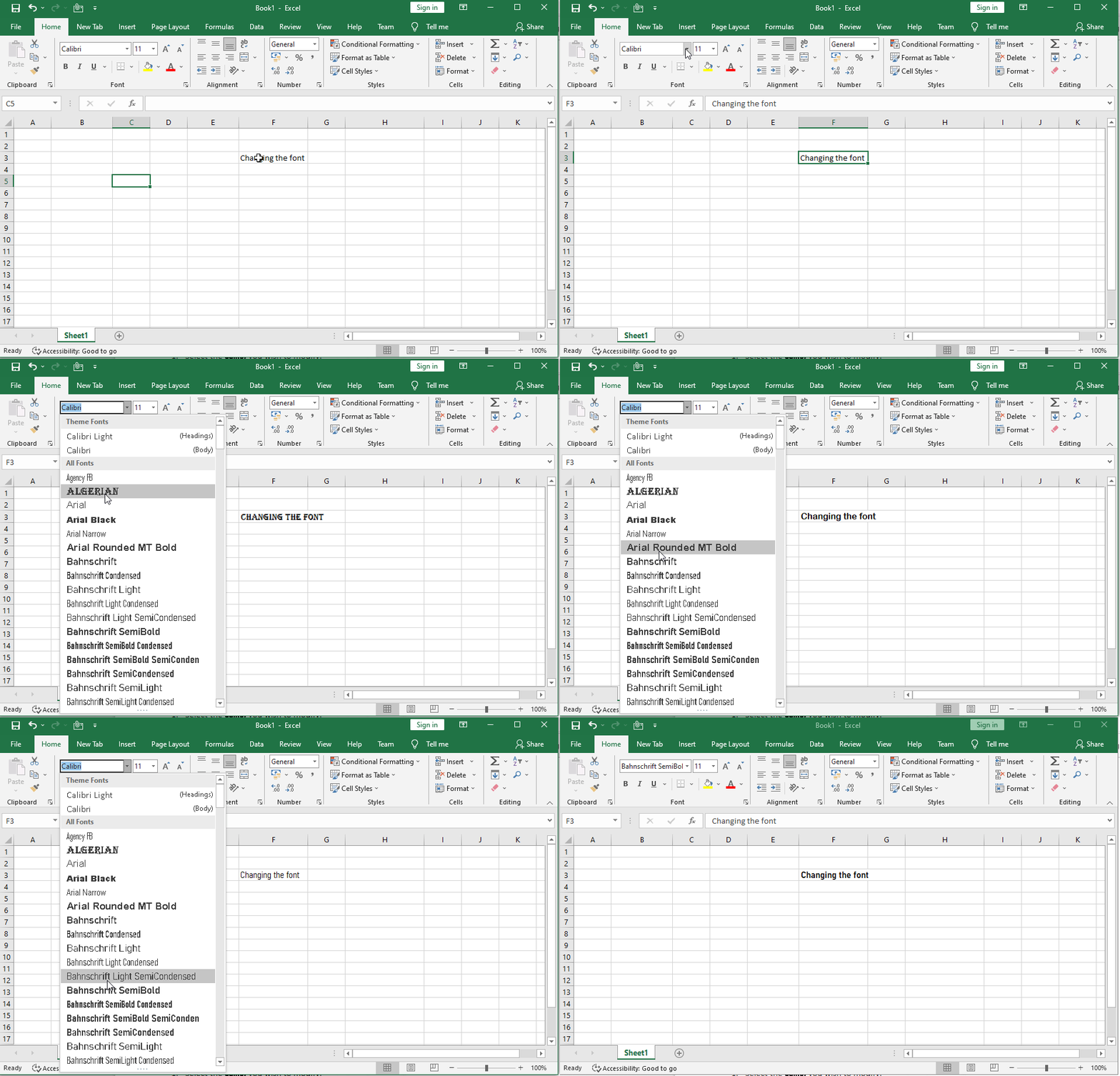
Note: When developing a workbook at the workplace, choose a typeface that is easy to read. Standard reading typefaces, in addition to Calibri, include Cambria, Times New Roman, and Arial.
To change the font size
We can change the font size as per our requirement. The minimum size of the font will be 8 and the maximum size of the font will be 72.
find below steps to change the font size
- Select the cell(s) you wish to modify.
- Click the drop-down arrow next to the Font Size command on the Home tab.
- The Font Size drop-down menu will appear.
- Select the desired font size.
- A live preview of the new font size will appear as you hover the mouse over different options.
- The text will change to the selected font size.
- Press enter to exist.

Note: You may also utilise the Increase Font Size and Decrease Font Size commands, or use your keyboard to input a custom font size.
To change the font colour and fill Colour
To emphasise essential facts or add aesthetic impact to a spreadsheet, you may alter the font colour of cell contents or the background colour of cells.
Find below steps to change the font colour
- Select the cell(s) to be modified.
- On the Home tab, select the Font Color command by clicking the drop-down arrow next to it. The Color menu will display.
- Choose the desired font color. When we hover the cursor over different color selections, a live preview of the new font color will show.
- The text will be changed to the font color you have chosen.

Find below steps to change the fill colour
- Select the cell to be formatted.
- In the Font group on the Home tab, click the Fill Color button to apply the most recently used colour.
- or click the Fill Color arrow to pick a new colour from the colour palette.

Note: To remove the fill colour from a chosen cell, click the Fill Color arrow and then No Fill in the palette.
Applying Font Styles in Excel
To highlight essential data in a spreadsheet, you may use one or more font styles. Font styles include characteristics such as bold, italic, and underline.
The characters become darker as they become more daring. The characters are slanted to the right when they are italicized. Underlining inserts a line below the cell contents rather than the cell itself.
To use the Bold, Italic, and Underline commands
- Select the cell(s) you want to change.
- On the Home tab, select the Bold (B), Italic (I), or Underline (U) command.
- In this example, we’ll make the text in the cell Bold, Italic, and Single Underline.
- To use a double underline, click the Underline arrow, then Double Underline from the menu.
- The chosen style will be used in the text.
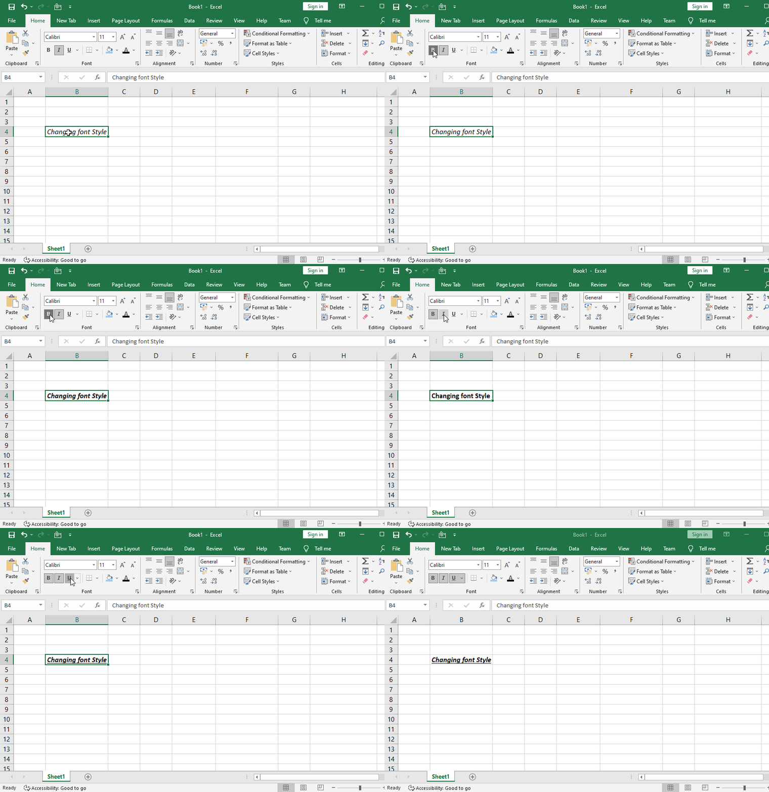
Note: You can also press Ctrl+B on your keyboard to make selected text bold, Ctrl+I to apply italics, and Ctrl+U to apply an underline.
Adding Cell Borders
Borders can be added to any or all sides of a single cell or range. Excel 2019 comes with a number of predefined border styles that you may utilise.
Fing below steps to add cell borders:
- Begin by selecting the cell to which you wish to add boundaries.
- In the Font group on the Home tab, click the Borders button to apply the most recently used border.
- Or click the Borders arrow to pick a new border from the menu.
- We can change the border color and style of the border. (See options in below image)

Note: To remove all borders from a chosen cell, click the Borders arrow and choose No Border from the menu. With the Draw Borders tools at the bottom of the Borders drop-down menu, you may draw borders and adjust their line style and colour.
Formatting Numbers in cell
Number formats can be applied to cells holding numbers to better reflect the sort of data they represent.
For example, You can show a numeric number as a percentage, currency, date or time, and so on.
The Number group on the Home tab of the Ribbon provides the most frequently used number formatting instructions .
You may also format numbers by opening the Format Cells dialogue box by selecting the dialogue box launcher in the Number group.

Note: Formatting has no effect on the actual value recorded in a cell. When a cell is chosen, the real value is utilised in computations and presented in the Formula bar.
Find below steps to format numbers
- Select the cell to be formatted.
- Perform one of the following actions on the Home tab, in the Number group:
Accounting Number
Format
To show the number with a dollar sign, comma separators, and two decimal places, click the Accounting Number Format button.
Note: You may change the currency symbol by clicking the Accounting Number Format arrow and then selecting the desired symbol from the drop-down box.
Percent Style
Click the Percent Style button
to convert the number to a
percentage and display it with a
percent sign and no decimal places.
Comma Style
Click the Comma Style button
to display the number with comma
separators and two decimal places.
Note: You can access additional
number formats by clicking the
Number Format arrow and selecting
the desired option from the menu

To modify the number of decimal places, do the following:
- Select the cell to be formatted.
- On the Home tab, under the Number group, select one of the following options.
- Increase the number of decimal places by clicking the Increase Decimal button.
- To reduce the number of decimal places, click the Decrease Decimal option.
Text Alignment
Any text input into your worksheet will be oriented to the bottom-left of a cell by default.
Any numbers will be aligned to the cell’s bottom-right corner.
Changing the orientation of your cell content allows you to choose how the material is shown in any cell, making it simpler to read.

To change horizontal text alignment
- Select the cell(s) you want to change.
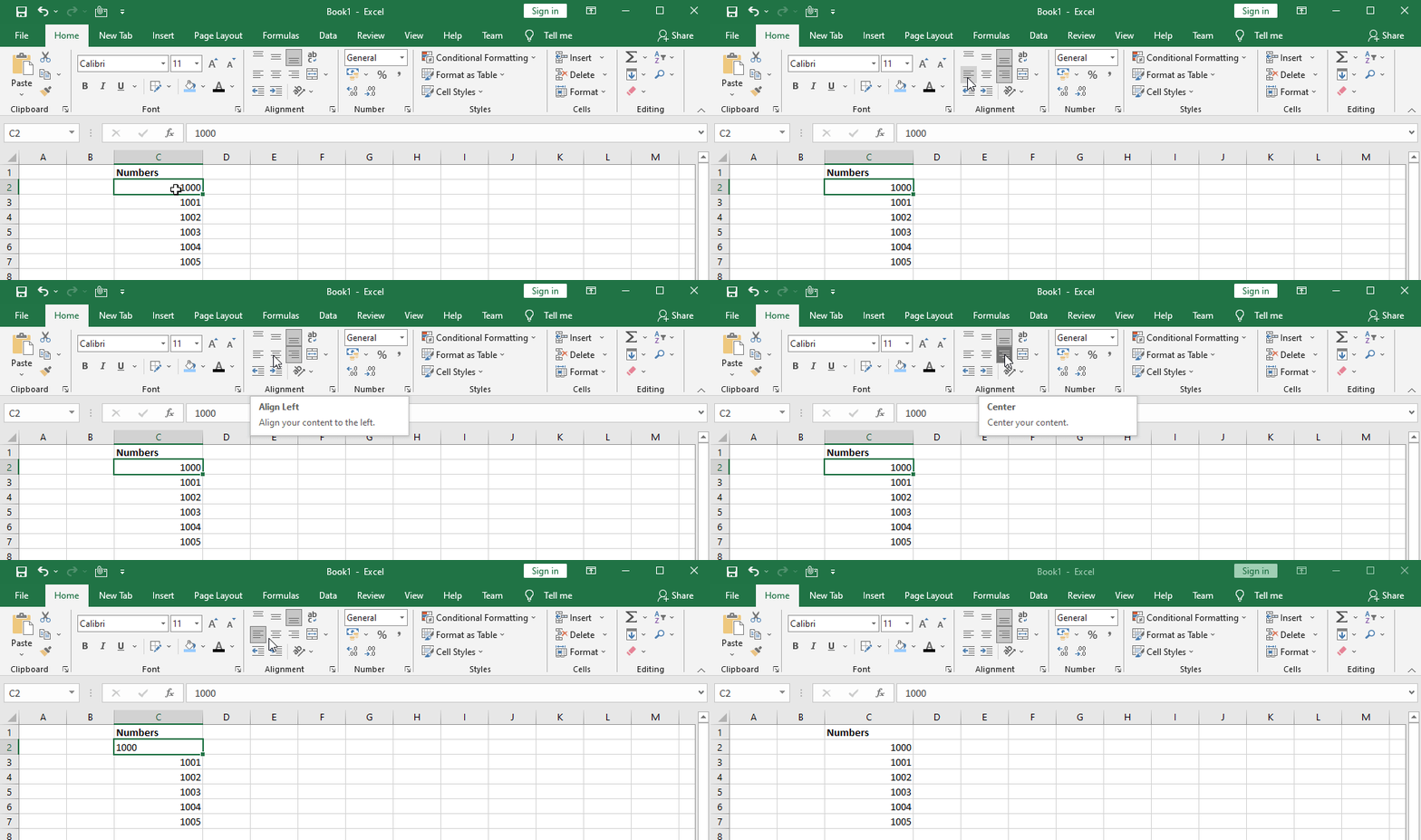
- On the Home tab, choose one of the three horizontal alignment commands. In this example, we’ll select Left Align.
- The three horizontal alignment commands are “Align Left”, “Center” and “Align Right“
- After selecting the LEFT Align command the text will realign itself.
To change vertical text alignment
- Select the cell(s) you want to change.
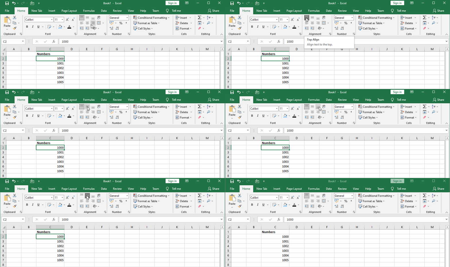
- On the Home tab, choose one of the three vertical alignment commands.
- The three Vertical alignment commands are “Top Align “, “Middle Align” and “Bottom Align“
- In this example, we’ll select TOP Align.
- After selecting the TOP Align command the text will realign itself.
Indenting Data
Indenting pulls data away from the cell’s edge. This is frequently used to denote a lower degree of importance (such as a subtopic)
Steps to Indenting Data
- Select the cell containing the information you wish to indent.
- In the Alignment group on the Home tab, click the Increase Indent button.
- Each click increases the indentation by one character.
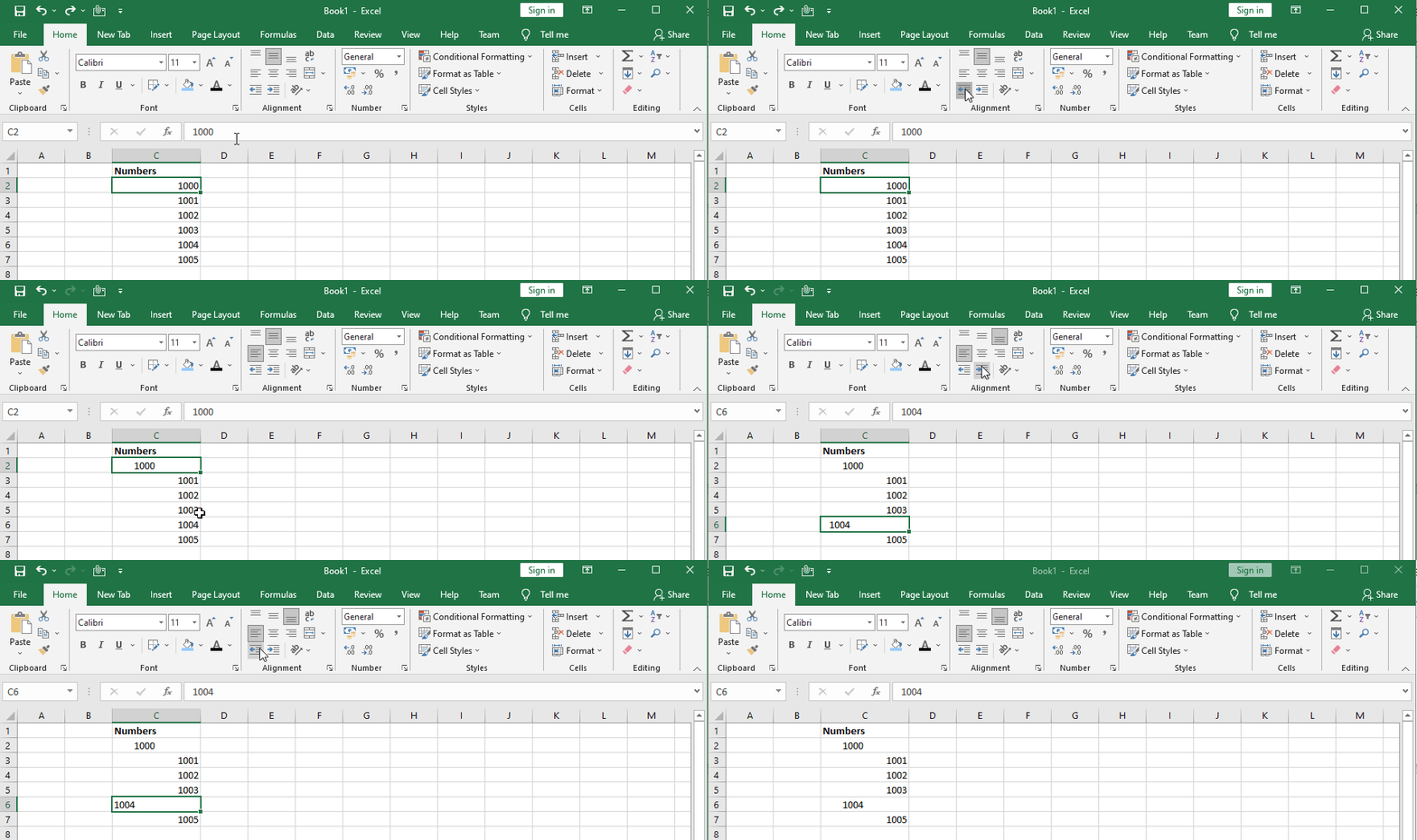
Note: The Lower Indent button in the Alignment group on the Home tab of the Ribbon may be used to decrease the indentation of data.
Rotating Data
Within a cell, you can rotate data clockwise, counterclockwise, or vertically. This is frequently used to mark narrow columns or to enhance the visual impact of a spreadsheet.
Steps to Rotating Data
- Select the cell containing the data to be rotated.
- On the Home tab, in the Alignment group, click the Orientation button and choose the appropriate choice from the menu.
- The row height adapts automatically to match the rotated data.

Note: By pressing the Orientation button and selecting the presently chosen orientation, you may return the data to its default orientation.
Wrapping Data
Wrapping allows you to show data on numerous lines within a cell. The number of wrapped lines is determined by the column width and the length of the data.
Steps to Wrapping Data
- Choose the cell containing the data you wish to wrap.
- In the Alignment group on the Home tab, select the Wrap Text option.
- The row height adapts automatically to match the wrapped data.

Note: By selecting the Wrap Text button again, you may return the data to its original format.
Merging Cells
Merging combines two or more adjacent cells into one larger cell. This is a great way to create
labels that span several columns.
Steps to Merging cells
- Choose the cells you wish to combine.
- On the Home tab, in the Alignment group, click the Merge & Center button to merge the chosen cells into one cell and center the data.
- Or click the Merge & Center arrow and choose one of the alternatives.
- Merge Across: Consolidates each row of the specified cells into a single bigger cell.
- Merge Cells: Combines the selected cells into a single cell.

Note: By clicking the Merge & Center arrow and then Unmerge Cells on the menu, you may divide a combined cell.
Copying Cell Formatting
You may copy the formatting of a single cell and paste it into additional cells in the worksheet. When numerous formats have been applied to a cell and you wish to format subsequent cells with all of the same formats, this can save you time and effort.
Steps to Copying Cell Formatting
- Select the cell containing the formatting that you wish to duplicate.
- In the Clipboard group on the Home tab, click the Format Painter button.
- The mouse cursor transforms into a plus symbol holding a paintbrush.
- Select the cell to which the copied formatting should be applied.

Note: If you wish to apply the copied formatting to more than one area, double-click the Format Painter button rather than just one. This activates the Format Painter until you press the Esc key.
Cell styles
Instead of manually formatting cells, you can use Excel’s predesigned cell styles. Cell styles are a quick and easy method to add professional formatting to various portions of your worksheet, such as titles and headers.
Steps to cell styling
- Select the cell(s) you wish to modify.
- Click the Cell Styles command on the Home tab, then choose the desired style from the drop-down menu.
- The selected cell style will appear.

Note: Except for text alignment, applying a cell style will overwrite any current cell formatting. If your workbook already has a lot of formatting, you might not want to employ cell styles.
THANK YOU FOR READING. PLEASE PROVIDE YOUR VALUABLE FEEDBACK.


Вывод из запоя: Какие услуги предоставляет наркологическая клиника
Вывести из запоя [url=https://vivodizzapoya.kz]https://vivodizzapoya.kz[/url] .
I gotta favorite this site it seems invaluable very useful
This really answered my problem, thank you!
I truly appreciate this post. I have been looking all over for this! Thank goodness I found it on Bing. You’ve made my day! Thanks again
With havin so much content do you ever run into any issues of plagorism or copyright infringement? My site has a lot of unique content I’ve either written myself or outsourced but it appears a lot of it is popping it up all over the web without my authorization. Do you know any methods to help reduce content from being ripped off? I’d definitely appreciate it.
Казино Чемпион 2024: Лучшие игры, бонусы и акции для игроков
Champion casino бездепозитный бонус [url=http://dk-slavniy.ru/]Champion casino бездепозитный бонус[/url] .
Наркология Самара: Профессиональное лечение зависимости
анонимная наркоклиника [url=https://narkolog-klinika-samara-1.ru/]https://narkolog-klinika-samara-1.ru/[/url] .
Как заработать на трэптоксе быстро и легко, Подробный обзор трэптокса и его возможностей
Трэптокс для шеи [url=https://www.epilstudio.ru/services/traptox/]https://www.epilstudio.ru/services/traptox/[/url] .
“Безопасность Трэптокс”. “Процедуры Трэптокс у доктора Шестаковой Татьяны Викторовны проводятся с соблюдением всех стандартов безопасности.”
“Question”. “Treptox safety?”
“Answer”. “Treptox procedures with Dr. Tatiana Shestakova are performed in compliance with all safety standards.”
I want to show you one exclusive program called (BTC PROFIT SEARCH AND MINING PHRASES), which can make you a rich man!
This program searches for Bitcoin wallets with a balance, and tries to find a secret phrase for them to get full access to the lost wallet!
Run the program and wait, and in order to increase your chances, install the program on all computers available to you, at work, with your friends, with your relatives, you can also ask your classmates to use the program, so your chances will increase tenfold!
Remember the more computers you use, the higher your chances of getting the treasure!
DOWNLOAD FOR FREE
Telegram:
https://t.me/btc_profit_search
Большой выбор запчастей МТЗ: Быстрая отправка и отличные цены
магазин запчастей мтз [url=http://www.zapchasty-mtz.ru/]http://www.zapchasty-mtz.ru/[/url] .