What is functions in Excel

A function is a preset formula that conducts computations based on certain data in a specific order.
Excel has several common functions that may be used to rapidly find the total, average, count, and so on.
Maximum and lowest values for a set of cells To utilize functions appropriately, you must first understand what they are.

Comprehend the many components of a function and how to build parameters to compute values and cell

Example: 
Formula =A1+A2+A3+A4+A5
Function =SUM(A1:A5)

Syntax of Function

A function must be written in a certain way in order to work properly, which is known as syntax.

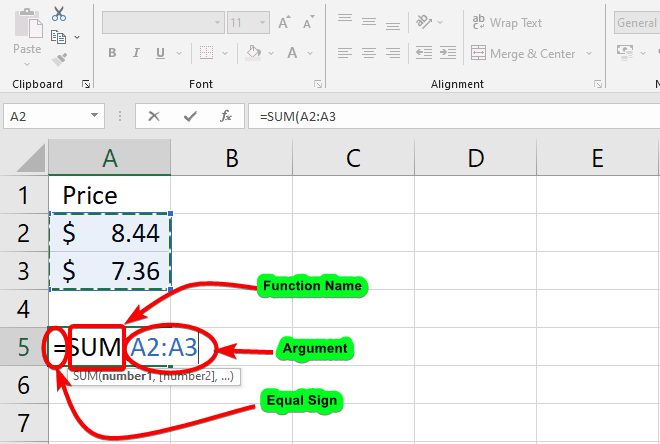
A function’s fundamental syntax consists of an equals sign (=), the function name (for example, SUM), and one or more Arguments. Arguments include the data you wish to compute.

=SUM(A2:A3)

Working with arguments in Functions

Arguments must be contained in parenthesis and can refer to both individual cells and cell ranges. Depending on the syntax required for the function, you can provide one or more parameters.

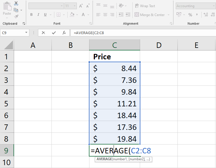
The function =AVERAGE(C2:C8), for example, would compute the average of the values in the cell range C2:C8. There is just one parameter to this function.

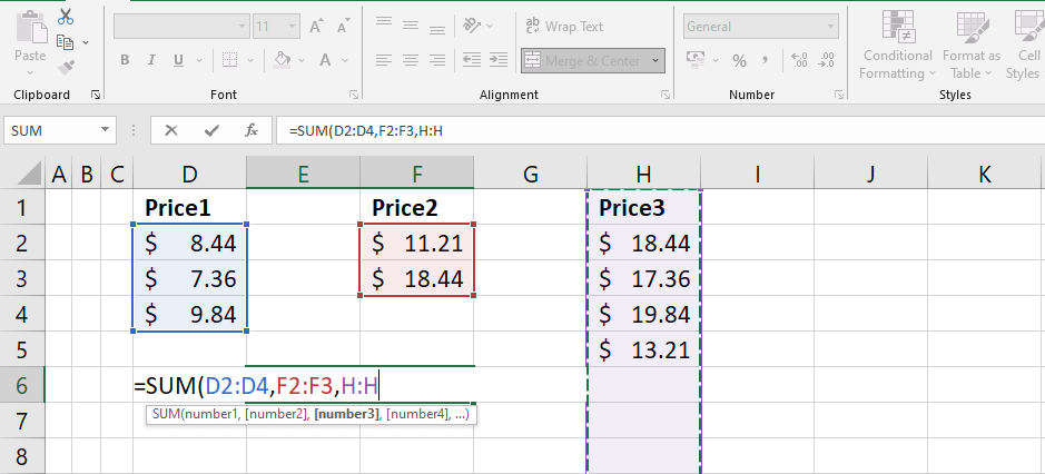
A comma must be used to separate several parameters. The function =SUM(A1:A3, C1:C2, E2), for example, will sum the values of all the cells in the three parameters.

How to create a function

Excel offers a wide range of features at your disposal. Here are some of the most commonly used functions:

1. SUM: This function adds all of the values in the argument’s cells. Example: =SUM(B2:B4)
2. COUNT: This function counts the number of cells in the argument that contain numerical data. This function is handy for rapidly calculating the number of objects in a cell range. Example: =COUNT(B2:B4)
3. AVERAGE: This function computes the average of the values in the input. It adds up the cells and divides the result by the number of cells in the argument. Example: =AVERAGE(B2:B4)
4. MAX: This function returns the cell value with the highest value in the parameter. Example: =MAX(B2:B4)
5. MIN: This method returns the lowest cell value in the parameter. Example: =MIN(B2:B4)

Creating a Basic Function

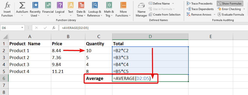
In the following example, we’ll use the AVERAGE function to construct a simple function that calculates the average price per unit for a list of recently ordered goods.

1. Choose the cell that will house the function.
2. Enter the required function name and the equals symbol (=). You may also choose the appropriate function from the list of recommended functions that appears underneath the cell as you enter. In our case, we’ll use =AVERAGE.
3. Within parentheses, enter the cell range for the argument. In this case, we’ll type (D2:D5).
4. On your keyboard, press Enter. The function will be computed, and the outcome will be shown in the cell.

When using functions, keep the following guidelines in mind:

1. The function expects arguments to be supplied in the order specified by the function.
2. Commas must be used to separate arguments.
3. Optional arguments must come after mandatory arguments.
4. Parentheses are required for all functions, including those with no parameters.

Using AutoSum command to create a Function

The AutoSum button allows you to quickly access the most frequently used functions (SUM, AVERAGE, COUNT, MAX, and MIN).

It may be found on the Ribbon’s Home and Formulas tabs.

The SUM function is the default action of the AutoSum button; you may access the other functions by pressing the arrow on the button (see Figure 5).

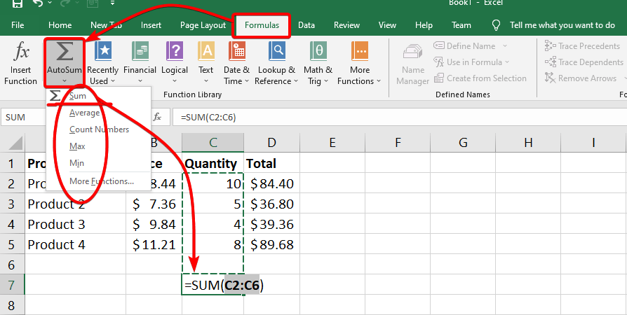
Example of AutoSum command

In our example below, we’ll create a function to calculate the total cost for a list of recently ordered items using the SUM function.

1. Choose the cell that will house the function.
2. On the Home tab, in the Editing group, find and click the arrow next to the AutoSum comman.
3. Then select the desired function from the drop-down menu.
4. In this example, we’ll use Sum.
5. The chosen function will be shown in the cell.
6. The AutoSum command will automatically choose a cell range for the parameter if it is positioned logically.
7. You may also specify the required cell range directly into the argument.
8. On your keyboard, press Enter.

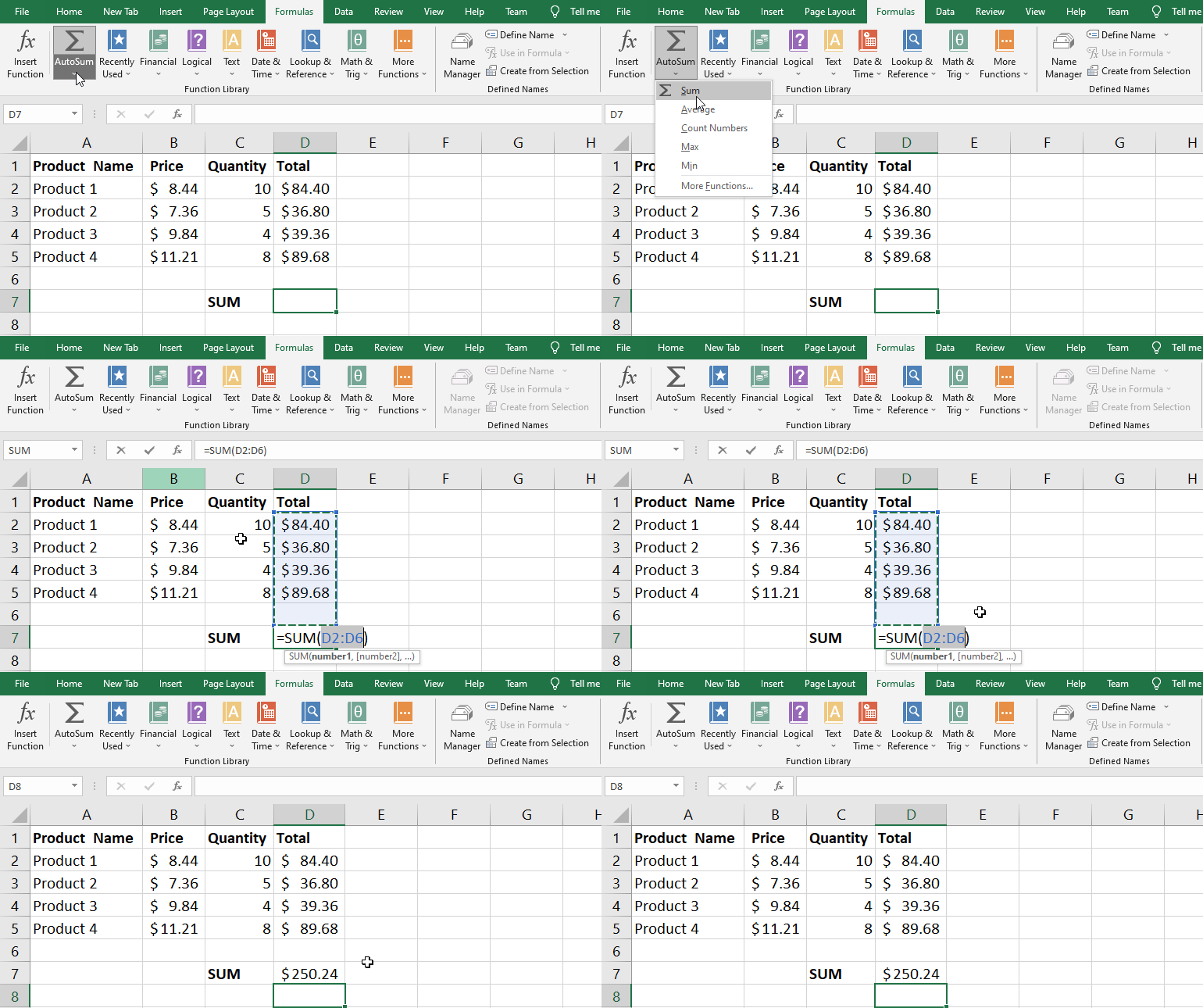
The Function Library in Excel

While Excel has hundreds of functions, the ones you use the most depend on the type of data in your workbooks.

There is no need to master every single function, but becoming acquainted with some of the many sorts of functions can be beneficial as you develop new applications.

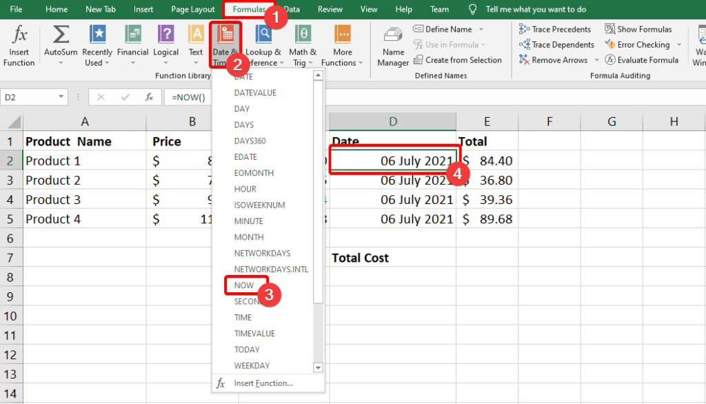
From the Function Library on the Formulas page, you may search for functions by category, such as Financial, Logical, Text, Date & Time, and more.

Note: Select the Formulas tab on the Ribbon to open the Function Library. The Function Library will be shown.

Componants of Function Library

Note: More Functions contains additional functions under categories for Statistical, Engineering, Cube,  Information, and Compatibility.

To insert a function from the Function Library

We can insert functions directly from the function library as we required. See steps below:

1. Select the cell that will contain the function.
2. Open the Function Library by clicking the Formulas tab on the Ribbon.
3. Select the required function category from the Function Library group.
4. From the drop-down menu, select the appropriate function.
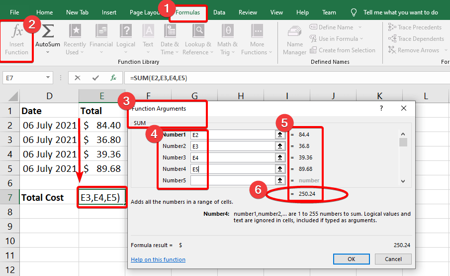
5. A dialogue box titled Function Arguments will open.
6. You’ll be able to input or choose the cells that will make up the parameters in the function from here.
7. Click OK after you’re finished with the arguments.
8. The function will be computed, and the outcome will be shown in the cell.

Note: Functions, like formulae, can be copied to neighbouring cells. Hover the mouse over the function cell, then click, hold, and drag the fill handle over the cells you want to fill. The function will be duplicated, and the values for those cells will be computed in relation to their rows or columns.

What is the Insert Function command

If you can’t find the correct function, you may use the Insert Function command to search for it using keywords.

While highly valuable, this command can be a bit tricky to use at times.

If you don’t have much expertise with functions, you might be better off perusing the Function Library.

However, for more sophisticated users, the Insert Function command can be a great tool to rapidly discover a function.

Steps to use the Insert Function command

Find the steps given below to insert a function from the “Insert function” command.

1. Choose the cell that will house the function.
2. On the Ribbon, pick the Formulas tab, then the Insert Function command.
3. A dialogue box titled Insert Function will open.
4. Enter a few terms that describe the computation you want the function to execute, then press the Go button.
5. Scroll through the results until you find the required function, then click OK.
6. The dialogue box Function Arguments will display.
7. When you’re done, click OK.
8. The function will be computed, and the outcome will be shown in the cell.

Enjoy!! Happy Learning…👍

THANK YOU FOR READING. PLEASE PROVIDE YOUR VALUABLE FEEDBACK.