Easy Excel Time-Savers
Excel Time-Savers – 5 Hidden Features for Busy People
Are you tired of wasting hours on tedious Excel tasks? Do you wish you had more time to focus on the important stuff? Well, you’re in luck Today, we’re going to uncover 5 hidden Excel features that will save you time, increase your productivity, and make you a rockstar in the world of spreadsheets.
What’s the Big Deal About Excel Time-Savers?
Let’s face it, Excel can be overwhelming, especially for beginners. With so many features and functions, it’s easy to get lost in the sea of possibilities. But, what if I told you that there are some secret features that can simplify your workflow, automate tasks, and give you back hours of your precious time?
Feature #1: Flash Fill – The Ultimate Time-Saver
Imagine having to manually enter hundreds of names, addresses, or phone numbers into your Excel spreadsheet. Sounds like a nightmare, right? That’s where Flash Fill comes in. This hidden gem can automatically fill in entire columns of data with just a few clicks.
How to Use Flash Fill:
- Select the cell range you want to fill.
- Go to the Data tab and click on Flash Fill.
- Excel will automatically detect the pattern and fill in the rest of the cells.
Example:
Suppose you have a list of names in column A, and you want to extract the first names only. With Flash Fill, you can do this in seconds.
| Name | First Name |
|---|---|
| John Smith | |
| Jane Doe | |
| Bob Johnson |
Select the cell range A1:A3, go to the Data tab, and click on Flash Fill. Excel will automatically fill in the first names in column B.
Feature #2: Power Query – The Data Manipulation Master
Power Query is a powerful tool that allows you to manipulate and transform your data with ease. With Power Query, you can merge data from multiple sources, remove duplicates, and perform complex calculations in a few clicks.
How to Use Power Query:
- Go to the Data tab and click on New Query.
- Select the data source you want to work with.
- Use the Power Query editor to manipulate and transform your data.
Example:
Suppose you have two tables with sales data from different regions. You want to merge the data and calculate the total sales for each region. With Power Query, you can do this in minutes.
Table 1:
| Region | Sales |
|---|---|
| North | 1000 |
| South | 2000 |
| East | 3000 |
Table 2:
| Region | Sales |
|---|---|
| West | 4000 |
| North | 5000 |
| South | 6000 |
Use Power Query to merge the two tables and calculate the total sales for each region.
Feature #3: Conditional Formatting with Formulas
Conditional formatting is a powerful tool that allows you to highlight important data in your spreadsheet. But, did you know that you can use formulas to take your conditional formatting to the next level?
How to Use Conditional Formatting with Formulas:
- Select the cell range you want to format.
- Go to the Home tab and click on Conditional Formatting.
- Select New Rule and choose Use a formula to determine which cells to format.
- Enter the formula you want to use to format the cells.
Example:
Suppose you want to highlight cells that contain the word “Error” in a column. You can use the following formula:
=A1:A10="Error"
Feature #4: The Power of PivotTables
PivotTables are a powerful tool that allows you to summarize and analyze large datasets with ease. With PivotTables, you can rotate, filter, and group your data to gain valuable insights.
How to Use PivotTables:
- Select the cell range you want to analyze.
- Go to the Insert tab and click on PivotTable.
- Drag and drop the fields you want to analyze into the Rows, Columns, and Values areas.
Example:
Suppose you have a dataset with sales data from different regions and products. You want to analyze the sales data by region and product. With PivotTables, you can do this in minutes.
Feature #5: Macros – The Ultimate Automation Tool
Macros are a powerful tool that allows you to automate repetitive tasks in Excel. With macros, you can record a series of actions and play them back with a single click.
How to Use Macros:
- Go to the Developer tab and click on Record Macro.
- Perform the actions you want to automate.
- Click on Stop Recording to save the macro.
- Assign a shortcut key or button to run the macro.
Example:
Suppose you want to automate the process of formatting a report every month. You can record a macro to perform the following actions:
- Select the entire worksheet
- Apply a specific font and font size
- Align the text to the center
- Insert a header and footer
With macros, you can automate this process with a single click.
Conclusion:
There you have it – 5 hidden Excel features that will save you time, increase your productivity, and make you a rockstar in the world of spreadsheets. From Flash Fill to macros, these features will simplify your workflow, automate tasks, and give you back hours of your precious time.
What’s Next?
Now that you’ve learned about these 5 hidden Excel features, it’s time to put them into practice. Try out each feature and see how they can benefit your workflow. Remember, practice makes perfect, so don’t be afraid to experiment and try new things.