What is Excel Formula

The capacity to compute numerical data using formulae is one of Excel’s most powerful capabilities.

In a spreadsheet, formulas are utilized to do calculations. Every formula must start with an equal symbol (=).

Formulas can include the following components:

1. Values that remain constant (such as 5 or 100).
2. References to cells (such as A1 or A1:A3).
3. Operators (for example, + for addition or * for multiplication).
4. A list of functions (such as SUM or AVERAGE).

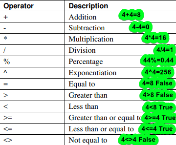
Operators in Excel’s Formula

Operators are mathematical symbols that represent certain operations.

Excel formulae support a wide range of operators (see Figure 1).

Arithmetic operators carry out fundamental mathematical operations (such as addition and subtraction) and provide numerical values.

When two values are compared, the comparison operator returns TRUE or FALSE.

Note: When a formula has more than one operator, Excel calculates from left to right in accordance with the conventional mathematical order of operations. This order can be changed by using parenthesis.computations within parentheses are done first.

The fundamental order of operations is as follows:

1. Percentage
2. Exponentiation
3. Division and Multiplication
4. Addition and subtraction
5. Comparison

1. Simple Excel Formula

Excel, like a calculator, can Add, Subtract, Multiply, and Divide numbers. We’ll learn here how to utilize cell references to build simple formulae in this session.

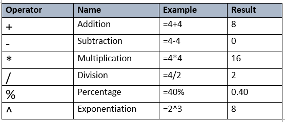
Mathematichal Operators in simple formula

For formulae, Excel employs conventional operators such as a plus symbol (+) for addition, a minus sign (-) for subtraction, an asterisk (*) for multiplication, a forward slash (/) for division, and a caret (^) for exponents.

In Excel, all formulae must begin with an equals symbol (=). This is due to the fact that the cell includes, or is equal to, the formula and the value it computes.

What is cell references

The majority of formulae are built via cell references.

A cell reference identifies a single cell or a group of cells.
There are three sorts of cell references: Relative, Absolute, and Mixture.

When a formula is transferred to other cells, these references act differently.

This is referred to as creating a cell reference. Because you may alter the value of referred cells without having to redo the calculation, using cell references ensures that your formulae are always accurate.

Note: Here note that cell reference could be entered manualy or we can select referenced cell's address by clicking on that cell.

Types of Cell References

Steps to create a formula

1. Choose the cell that will house the formula. Here A4 (See the below image).
2. Enter the equals sign (=) into the text box. Take note of how it looks in the cell as well as the formula bar.
3. In the formula, type the cell address of the cell you want to reference first: cell A1 in our example.
4. The mentioned cell will be surrounded by a blue border.
5. Enter the mathematical operation that you want to utilize. In this example, we’ll use the plus symbol (+).
6. In the formula, type the cell address of the cell you want to reference second: cell A2 in our case. The mentioned cell will be surrounded by a red border.
7. On your keyboard, press Enter. The formula will be computed, and the result will be shown in the cell.

Note:  If the result of a formula is too large to fit in a cell, it will be shown as pound marks (#######) instead of a value. This indicates that the column is too narrow to display the cell content. To display the cell content, just raise the column width.
The formula will be shown in both the cell and the formula bar.

Modifying values with cell references

The actual benefit of cell references is that they allow you to alter data in your spreadsheet without rewriting the formula.

Steps to Modifying a formula

1. Selct a cell in which formula is applied.
2. Now select referenced cell then click on new referenced cell from where we want to update the data.
3. Repeat same process for other refrences cells if you want to change them all.
4. We can change single or multiple referenced cells as required.
5. And then click Enter to find new updated value.
6. See below Figure, Here we are updating Formula in cell A3 by changing referenced cells A1 to C1 and A2 to C2.

Note: Excel will not always inform you if your formula includes a mistake, therefore it is your responsibility to double-check all of your formulae.

How to edit a formula

You may wish to change an existing formula from time to time. We’ve put an erroneous cell address in our formula in the example below, so we’ll need to change it.

Actually, this is a similar process as mentioned above (Modifying values with cell references).

Steps to edit a formula

1. Select the cell that contains the formula you want to change.
2. To change the formula, click the formula bar.
3. You may also examine and change the formula right within the cell by double-clicking it.
4. Any referenced cells will be surrounded by a border.
5. When you’re finished, press Enter on your keyboard or choose the Enter option from the formula bar.
6. The formula is changed, and the new value is presented in the cell.

Note: If you change your mind, you may cancel your formula by using the Esc key on your computer or clicking the Cancel command on the formula bar.

Note: Hold the Ctrl key and hit (grave accent) to see all of the formulae in a spreadsheet. The grave accent key is commonly found in the upper-left region of the keyboard. You may return to the usual view by pressing Ctrl+ again.

How to Display Formulas

Cells containing formulae display the formula’s results rather than the formula itself.

By choosing specific cells and glancing at the Formula bar, you can examine the underlying formulae.

Making all of the formulas in a worksheet accessible is another method to see them.

To display all formulas:

Click the Show Formulas button on the Formulas tab, in the Formula Auditing group. To fit the formulae, the width of each column is increased.

2. Complex Excel Formulas

A simple formula is a mathematical expression that contains only one operator, such as 8+4.

A complex formula, such as 8+4*7, contains more than one mathematical operator.

When a formula contains more than one operation, the order of operations tells Excel which operation to calculate first.

In order to calculate complex formulas, you must first understand the order of operations.

The sequence of events

Excel computes formulas in the following order of operations:

1. Operations surrounded by parentheses
2. Exponential calculations (e.g., 4^2)
3. Division and multiplication, whichever comes first
4. Subtraction and addition, whichever comes first

Creating complicated formula 

In the next example, we will show how Excel solves a complicated formula using the sequence of operations.

In this case, we wish to compute the cost of sales tax for an invoice.

In cell D4, we’ll write our formula as =(D2+D3)*0.075.

To determine the cost of sales tax, we will put the costs of our products together and then multiply that total by the 7.5 percent tax rate (which is printed as 0.075).

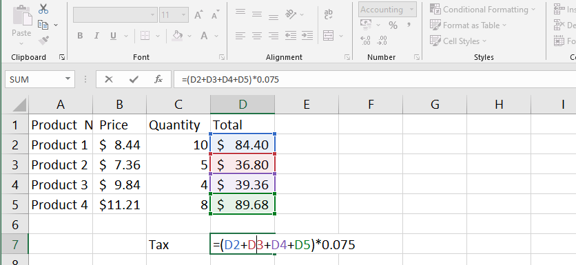
Note: It is critical to input complicated formulae in the right order of operations.
 Otherwise, Excel will not produce correct results. If the parenthesis are not present in our example, the multiplication is computed first, and the result is wrong. Parentheses are the most effective technique to specify which computations in Excel will be done first.

Enjoy!! Happy Learning…👍

THANK YOU FOR READING. PLEASE PROVIDE YOUR VALUABLE FEEDBACK.